EPA (expected points added) is being used too much. There, I said it. Hear me out before you revoke my analytics club membership. I also want to state that no single application of EPA has driven me to this conclusion but rather many over the years including my own work quantifying player value using Bayesian models that uses EPA to estimate player value! From scrutinizing my own work and others I’ve come to the conclusion that EPA’s use as an evaluation tool should be limited largely to team drives and games, complete quarterback seasons, league-wide trends, and to inform other models like win probability. Use of EPA to evaluate per play averages in many specific game situations, in my opinion, should be discontinued.

Virgil Carter & Robert Machol’s attempt to frame football in terms of expected points was revolutionary and perhaps the first influential sports analytics paper despite it being ignored for about 40 years. Thanks to Brian Burke’s site and then later work to make expected points models public (driven largely by Ron Yurko and Ben Baldwin), expected points and EPA as a way to analyze football has finally become mainstream. I remember the first time I heard my ESPN colleague (at the time) Domonique Foxworth casually use “EPA” without explanation on Around the Horn and I couldn’t stop smiling from my cubicle. We won!

Humility

We should all be more quick to acknowledge flaws with any metric and EPA is far from perfect. Work by UPenn PhD student Ryan Brill recently showed that expected points models are built on data rife with selection bias which can impact how confident we can be in 4th down decision models.

Distribution of EPA on a Play

EPA is the difference of between the expected net number of points the team will score before the play happens and then after the play happens. The problem is that the distribution of expected outcomes on a football play is anything but unimodal or symmetric let alone normally distributed. So when we use EPA, it doesn’t actually mean that a 0 EPA play on a play is the 50th percentile outcome. Sometimes 0 EPA is well above the 50th percentile outcome, and sometimes it is well below!

Let’s look at a few examples.

Changing Distributional Shape of EPA Outcomes

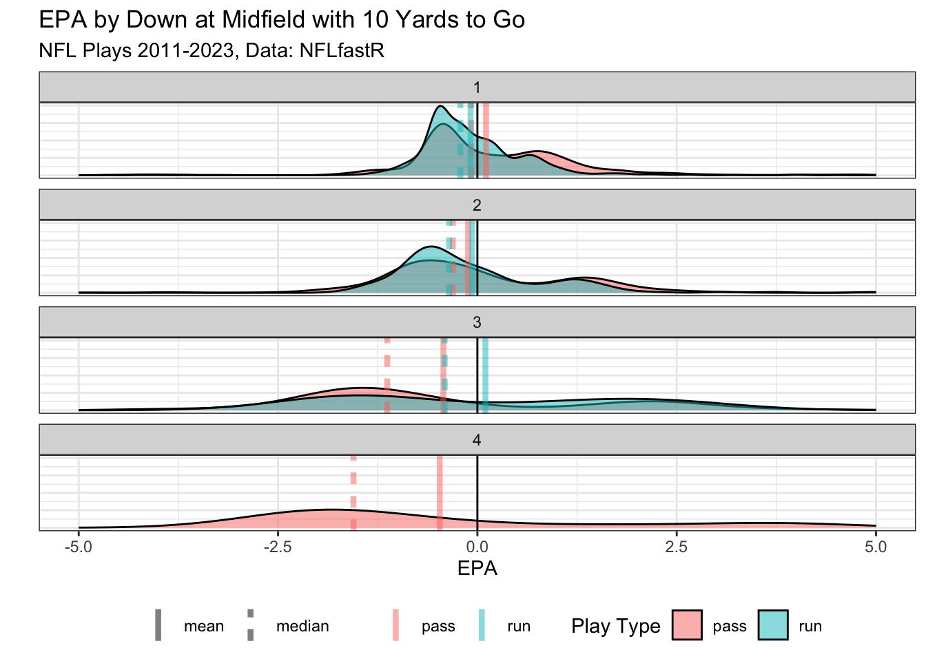
We’ll start with the empirical distribution of EPA for a pretty neutral situation at midfield for each down and play type (run & pass).

For each down there is a bimodal distribution of outcomes whose variance and skewness increase for each additional down. This matters because the means are pulled away from the center of the distribution towards the side of the skew. Players and teams that are in these situations will get credit or blame in terms of EPA for simply performing at the median or 50th percentile. For example a 50th percentile performance for a run on 3rd down and 10 at the 50 is worth -0.41 EPA despite it being simply the median outcome! If we are using EPA per play to compare players in certain situations and one player happened to be in this situation more than others then that alone will make them appear better.

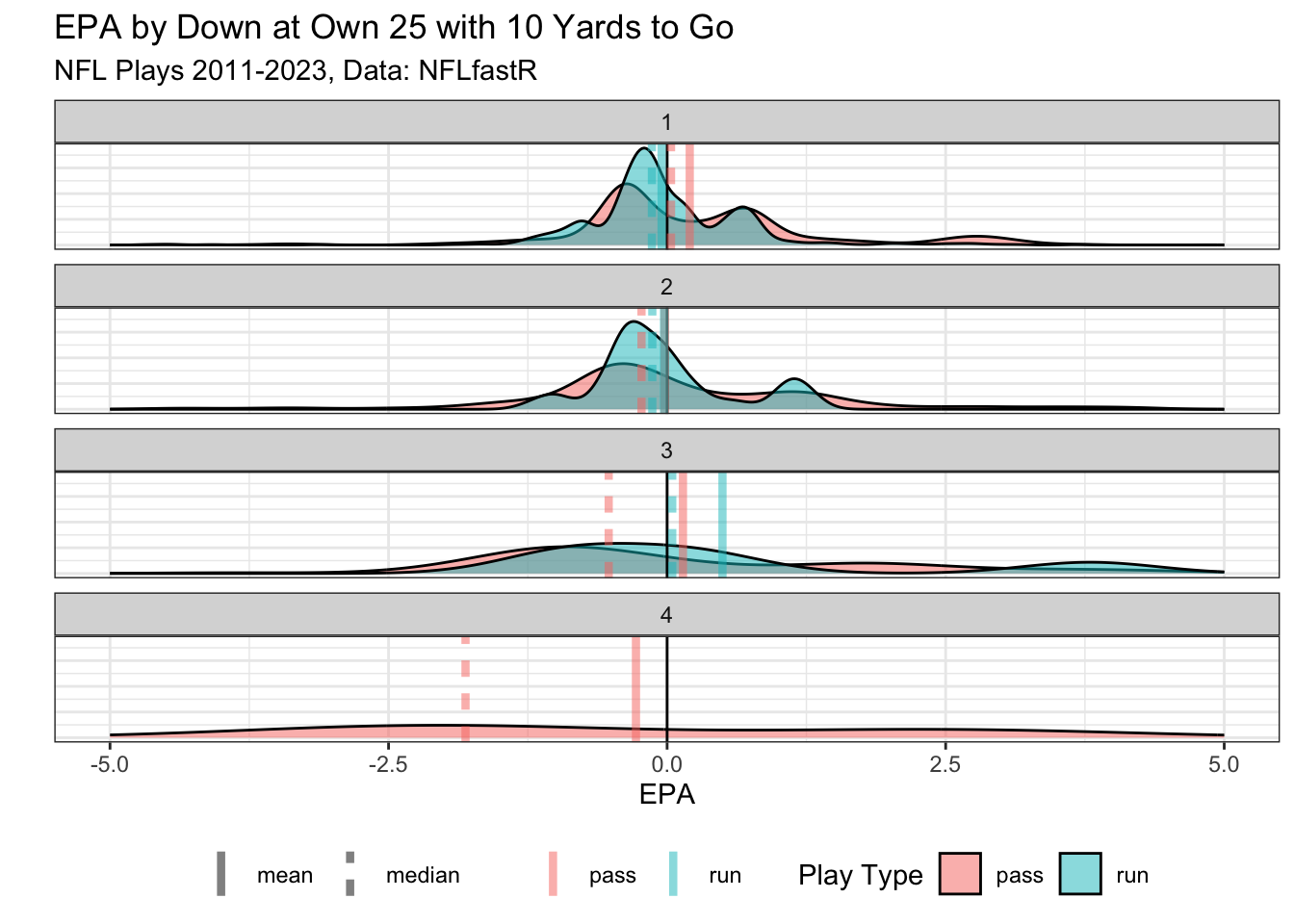
We can also look at the most common starting field position of the 25 yard line (usually after a kickoff).

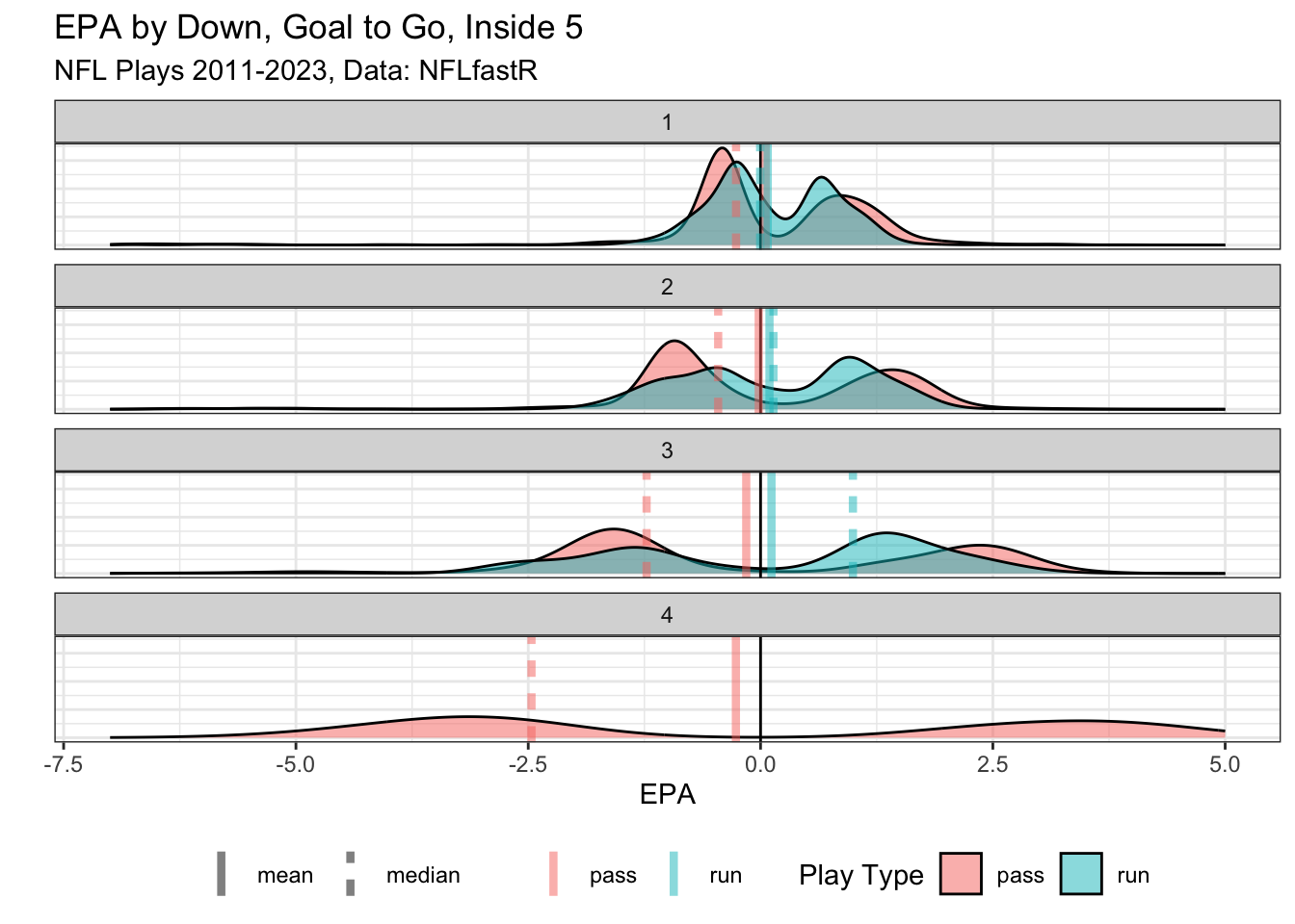
An even more extreme example of this, but still a common situation, is plays inside the 5 yard line in “goal to go” situations.

Player Credit

EPA is used often to compare player performances. In fact total EPA gained on the season for quarterbacks mirrors closely the results of the MVP voting. In recent years, several attempts have been made to assign credit to players based on how that player’s teams unit performs in terms of EPA (Paul Sabin Plus-Minus, PFF WAR, Yurko nflWAR, Baldwin EPA+CPOE composite, Kevin Cole Plus-Minus).

Barring extreme situations where a player intentionally gives himself up instead of scoring at the end of the game to preserve possession and ensure victory, or going out of bounds to stop the clock, the goal of each player on a football team on each play is to advance the ball as far as possible towards the end-zone (for the offense) and likewise to prevent that from happening for the defense.

This begs questions such as, do we use EPA as the preferred metric because it’s the best metric to encapsulate individual and team performance on a play, or do we use it simply because it isn’t yards? And why can’t we just use yards in some situations? Is the same metric preferable for the whole season as for a set of plays in specific situations?

Flaws of EPA

As I see it, EPA has three main flaws:

The large jump in EPA at the 1st down line vs 1 yard short of the first down line. That one additional yard is attained largely due to chance.
EPA does not follow a symmetric unimodal distribution, and depending on the situation it can skew left, skew right, be bimodal, unimodal, and more! This means that EPA per play for a team, unit, or player is affected largely by situation before the results of the play occur.
Selection Bias. Until recently all EPA models were built off observed plays. Better teams have more plays in the opposing territory, biasing the expectation towards better teams in those situations. Brill & Wyner 2024 use catalytic priors in an effort to adjust expected points models for this selection bias.

Yards vs EPA

We all know that 10 yards on 3rd and 10 and 10 yards on 3rd and 20 are not worth the same to the offensive team. We know EPA accounts for this problem.

Let’s consider the hypothetical situation, it is 3rd and 10 at exactly midfield in the 1st quarter of a 0-0 game.

Result A: The team gains 9 yards.
Result B: The team gains 10 yards.

Now in terms of EPA, according to the NFLFastR model, the Expected Points before the play is 1.71 while the EPA for Result A is -0.09 compared to result B of 2.02.

While in yards the team gained 10% more in situation B than A, in EPA one play is drastically different than the other. That is a massive difference for players with close to a coin flip difference in result. In causal inference we would call this spatial proximity. That means the difference of the play resulting in 9 yards vs 10 yards is mostly due to chance yet EPA results in a massive difference of that evaluation. If we are comparing players or teams in specific situations, our sample sizes can be overrun by these cliffs. If we do this as analysts we are making the same mistake fans make by overrating a team with an abundance of close wins.

Using Yards is OK

EPA is still useful in many situations and so are yards. In fact, in a lot of situations yards are a better evaluation tool than EPA. Plus yards are understood better by casual fans and decision makers than EPA is.

Let’s look at quarterbacks on 3rd down and less than 5 yards to go in the first half of games since 2011. I will include quarterback seasons with at least 25 snaps in this situation. I will also define Total Adjusted Net Yards as yards_gained + 20*touchdown - 45*turnover for all quarterback dropbacks (i.e. QB sacks, runs, and passes).

Avg. QB Performance on 3rd and 5 or less (1st Half)

2011-2023, data from NFLFastR

Sorted by EPA per play, the top of this list looks very reasonable. Patrick Mathomes, Jalen Hurts, and Peyton Manning are all at the top but then we get into some interesting names that we don’t typically think of when it comes to leading an NFL leaderboard of quarterbacks like Carson Wentz, Derek Carr, and Geno Smith.

Sure, these are smaller sample sizes because I’m filtering down, but this whole exercise is to examine what happens to EPA when we filter down. As analysts we make these comparisons or see others make these comparisons with similar sample sizes all the time!

Even though each season is a much smaller sample size, we can make some conclusions with almost 300 or so of these quarterback seasons available to us. We can look at the stability from how a quarterback does one season to the next on 3rd and less than 5.

Stat	Stability
EPA	0.002
TOT ANY	0.004
YDS	0.093

Small samples are noisy so none of these have high year to year correlation, but ~ 0.10 is still a lot higher than 0.003!

Why is this?

Well for a QB, over the course of a season, the benefits of accounting for yardline, down, distance, time remaining, etc. in EPA will make it more predictive than yards. The opposite can be true when we start splicing certain game situations. When we splice the data for certain situations in a game or for situations in a play that are correlated with situations in a game, using EPA may now hurt predictability because, among other things, the jump at the first down line coupled with small sample sizes. The goal of every team and player is to get as many yards as possible (with some very limited exceptions) so it is ok and can be preferable to use yards when we are honing in on specific situations.

Beyond Yards & EPA?

I believe the future of evaluation of players and teams goes beyond using yards, EPA, WPA (win probability added), or success rate. In order to truly quantify performance we need to understand where on the distribution of outcomes (accounting for the situation) the result of that play (or micro-play if using tracking data) falls. This is not trivial, and it is something I am actively working on. Want to help or be involved? Reach out!

--- title: "Slow Down Using EPA for Everything" date: 2024-01-05 author: "Paul Sabin" description: "Is using EPA always the best metric of choice? Occam's razor would suggest sometimes its best to stick with simpler measurements such as yards." categories: - football - sports analytics - EPA image: "img/card.png" twitter-card: image: "img/card.png" open-graph: image: "img/card.png" format: html editor: visual execute: echo: false warning: false error: false message: false --- ```{r} library(tidyverse) library(nflfastR) library(ggridges) library(gt) library(gtExtras) library(viridis) library(xgboost) # library(plotly) options(tibble.width = Inf) total_seasons <- 13 cross_validate <- FALSE#if true, run through and cross validate, if not fit model on all seasons nfl_schedule <- nflreadr::load_schedules() max_season <- max(nfl_schedule$season) all_seasons <- (max_season - total_seasons + 1):max_season nfl_pbp <- load_pbp(all_seasons) # player_yearly_salary <- get_nfl_player_contract_by_season(nfl_contracts) ## fix known bad "end_yardline" value nfl_pbp <- nfl_pbp %>% mutate(end_yard_line = replace(end_yard_line, end_yard_line == "GB -126", "GB 18")) nfl_pbp_simple <- nfl_pbp %>% mutate(half = ceiling(qtr / 2), loc = case_when(tolower(location) == "neutral" ~ "n", posteam == home_team ~ 'h', posteam == away_team ~ 'a', TRUE ~ NA_character_), turnover = if_else(fumble_lost == 1 | interception == 1, 1, 0), current_tot_score = posteam_score + defteam_score ) %>% dplyr::select(season, game_id, play_id, series, series_success, posteam, defteam, home_team, # away_team, play_type, special_teams_play, passer, passer_id, name, id,#generic if for passing & rushing qb_kneel, qb_spike, penalty, turnover, fumble_lost, interception, touchdown, pass_attempt, rush_attempt, roof, surface, temp, wind, yards_gained, current_tot_score, current_score_diff = score_differential, epa, ep, wpa, wp, vegas_wp, loc, # location, qb_dropback, half_seconds_remaining, half, qtr, yardline_100, down, ydstogo, play_clock, posteam_timeouts_remaining, defteam_timeouts_remaining ) ``` EPA (expected points added) is being used too much. There, I said it. Hear me out before you revoke my analytics club membership. I also want to state that no single application of EPA has driven me to this conclusion but rather many over the years including my own work [quantifying player value using Bayesian models](https://www.degruyter.com/document/doi/10.1515/jqas-2020-0033/html) that uses EPA to estimate player value! From scrutinizing my own work and others I've come to the conclusion that EPA's use as an evaluation tool should be limited largely to team drives and games, complete quarterback seasons, league-wide trends, and to inform other models like win probability. Use of EPA to evaluate per play averages in many specific game situations, in my opinion, should be discontinued. Virgil Carter & Robert Machol's attempt to frame football in terms of [expected points](https://pubsonline.informs.org/doi/abs/10.1287/opre.19.2.541) was revolutionary and perhaps the first influential sports analytics paper despite it being ignored for about 40 years. Thanks to Brian Burke's [site](https://www.advancedfootballanalytics.com/) and then later work to make expected points models public (driven largely by [Ron Yurko](https://scholar.google.com/citations?view_op=view_citation&hl=en&user=CBT7NWQAAAAJ&citation_for_view=CBT7NWQAAAAJ:IjCSPb-OGe4C) and [Ben Baldwin](https://www.nflfastr.com/)), expected points and EPA as a way to analyze football has finally become mainstream. I remember the first time I heard my ESPN colleague (at the time) Domonique Foxworth casually use "EPA" without explanation on *Around the Horn* and I couldn't stop smiling from my cubicle. We won! ## Humility We should all be more quick to acknowledge flaws with any metric and EPA is far from perfect. Work by UPenn PhD student Ryan Brill [recently](https://www.youtube.com/watch?v=uS4XxQ0LVfE) showed that expected points models are built on data rife with selection bias which can impact how confident we can be in 4th down decision models. ## Distribution of EPA on a Play EPA is the difference of between the expected net number of points the team will score before the play happens and then after the play happens. The problem is that the distribution of *expected* outcomes on a football play is anything but unimodal or symmetric let alone normally distributed. So when we use EPA, it doesn't actually mean that a 0 EPA play on a play is the 50th percentile outcome. Sometimes 0 EPA is well above the 50th percentile outcome, and sometimes it is well below! Let's look at a few examples. ### Changing Distributional Shape of EPA Outcomes We'll start with the empirical distribution of EPA for a pretty neutral situation at midfield for each down and play type (run & pass). ```{r} pbp_midfield <- nfl_pbp_simple %>% filter(yardline_100 == 50, (down <= 3 & play_type %in% c("pass", "run")) | down == 4 & play_type == "pass", ydstogo == 10 ) pbp_midfield_summary <- pbp_midfield %>% group_by(down, play_type) %>% summarize(mean_epa = mean(epa), median_epa = median(epa), plays = n() ) %>% ungroup() pbp_midfield_summary_long <- pbp_midfield_summary %>% pivot_longer(cols = ends_with("epa"), names_to = "stat", values_to = "epa") %>% mutate(stat = str_remove(stat, "_epa")) pbp_midfield %>% ggplot(aes(x = epa, fill = play_type, group = play_type) ) + geom_density(alpha = 0.5 ) + geom_vline(xintercept = 0) + geom_vline(data = pbp_midfield_summary_long, aes(xintercept = epa, linetype = stat, color = play_type ), alpha = 0.5, linewidth = 1.5 ) + xlim(-5, 5) + ylab("") + xlab("EPA") + theme_bw() + theme(legend.position = 'bottom', axis.ticks.y = element_blank(), axis.text.y = element_blank() ) + scale_fill_discrete("Play Type") + scale_color_discrete("") + scale_linetype_discrete("") + facet_wrap(~down, ncol = 1) + ggtitle("EPA by Down at Midfield with 10 Yards to Go", subtitle = paste0("NFL Plays ", min(nfl_pbp_simple$season), "-", max(nfl_pbp_simple$season), ", Data: NFLfastR" ) ) ``` For each down there is a bimodal distribution of outcomes whose variance and skewness increase for each additional down. This matters because the means are pulled away from the center of the distribution towards the side of the skew. Players and teams that are in these situations will get credit or blame in terms of EPA for simply performing at the median or 50th percentile. For example a 50th percentile performance for a run on 3rd down and 10 at the 50 is worth `r pbp_midfield_summary_long %>% filter(down == 3, play_type == "run", stat == "median") %>% pull(epa) %>% round(digits = 2)` EPA despite it being simply the median outcome! If we are using EPA per play to compare players in certain situations and one player happened to be in this situation more than others then that alone will make them appear better. We can also look at the most common starting field position of the 25 yard line (usually after a kickoff). ```{r} pbp_25 <- nfl_pbp_simple %>% filter(yardline_100 == 25, (down <= 3 & play_type %in% c("pass", "run")) | down == 4 & play_type == "pass", ydstogo == 10 ) pbp_25_summary <- pbp_25 %>% group_by(down, play_type) %>% summarize(mean_epa = mean(epa), median_epa = median(epa), plays = n() ) %>% ungroup() pbp_25_summary_long <- pbp_25_summary %>% pivot_longer(cols = ends_with("epa"), names_to = "stat", values_to = "epa") %>% mutate(stat = str_remove(stat, "_epa")) pbp_25 %>% ggplot(aes(x = epa, fill = play_type, group = play_type) ) + geom_density(alpha = 0.5 ) + geom_vline(xintercept = 0) + geom_vline(data = pbp_25_summary_long, aes(xintercept = epa, linetype = stat, color = play_type ), alpha = 0.5, linewidth = 1.5 ) + xlim(-5, 5) + ylab("") + xlab("EPA") + theme_bw() + theme(legend.position = 'bottom', axis.ticks.y = element_blank(), axis.text.y = element_blank() ) + scale_fill_discrete("Play Type") + scale_color_discrete("") + scale_linetype_discrete("") + facet_wrap(~down, ncol = 1) + ggtitle("EPA by Down at Own 25 with 10 Yards to Go", subtitle = paste0("NFL Plays ", min(nfl_pbp_simple$season), "-", max(nfl_pbp_simple$season), ", Data: NFLfastR" ) ) ``` An even more extreme example of this, but still a common situation, is plays inside the 5 yard line in "goal to go" situations. ```{r} pbp_goaltogo <- nfl_pbp_simple %>% filter(yardline_100 <= 5, (down <= 3 & play_type %in% c("pass", "run")) | down == 4 & play_type == "pass", ydstogo <= yardline_100 ) pbp_goaltogo_summary <- pbp_goaltogo %>% group_by(down, play_type) %>% summarize(mean_epa = mean(epa), median_epa = median(epa), plays = n() ) %>% ungroup() pbp_goaltogo_summary_long <- pbp_goaltogo_summary %>% pivot_longer(cols = ends_with("epa"), names_to = "stat", values_to = "epa") %>% mutate(stat = str_remove(stat, "_epa")) pbp_goaltogo %>% ggplot(aes(x = epa, fill = play_type, group = play_type) ) + geom_density(alpha = 0.5 ) + geom_vline(xintercept = 0) + geom_vline(data = pbp_goaltogo_summary_long, aes(xintercept = epa, linetype = stat, color = play_type ), alpha = 0.5, linewidth = 1.5 ) + xlim(-7, 5) + ylab("") + xlab("EPA") + theme_bw() + theme(legend.position = 'bottom', axis.ticks.y = element_blank(), axis.text.y = element_blank() ) + scale_fill_discrete("Play Type") + scale_color_discrete("") + scale_linetype_discrete("") + facet_wrap(~down, ncol = 1) + ggtitle("EPA by Down, Goal to Go, Inside 5", subtitle = paste0("NFL Plays ", min(nfl_pbp_simple$season), "-", max(nfl_pbp_simple$season), ", Data: NFLfastR" ) ) ``` ## Player Credit EPA is used often to compare player performances. In fact total EPA gained on the season for quarterbacks mirrors closely the results of the [MVP voting](https://www.reddit.com/r/nfl/comments/rkppy0/oc_the_mvp_race_and_epa/). In recent years, several attempts have been made to assign credit to players based on how that player's teams unit performs in terms of EPA (*Paul Sabin Plus-Minus, PFF WAR, Yurko nflWAR, Baldwin EPA+CPOE composite, Kevin Cole Plus-Minus*). Barring extreme situations where a player intentionally gives himself up instead of scoring at the end of the game to preserve possession and ensure victory, or going out of bounds to stop the clock, the goal of each player on a football team on each play is to advance the ball as far as possible towards the end-zone (*for the offense*) and likewise to prevent that from happening for the defense. This begs questions such as, do we use EPA as the preferred metric because it's the best metric to encapsulate individual and team performance on a play, or do we use it simply because it isn't *yards*? And why can't we just use yards in some situations? Is the same metric preferable for the whole season as for a set of plays in specific situations? # Flaws of EPA As I see it, EPA has three main flaws: 1. The large jump in EPA at the 1st down line vs 1 yard short of the first down line. That one additional yard is attained largely due to chance. 2. EPA does not follow a symmetric unimodal distribution, and depending on the situation it can skew left, skew right, be bimodal, unimodal, and more! This means that EPA per play for a team, unit, or player is affected largely by situation before the results of the play occur. 3. Selection Bias. Until recently all EPA models were built off observed plays. Better teams have more plays in the opposing territory, biasing the expectation towards better teams in those situations. Brill & Wyner 2024 use catalytic priors in an effort to adjust expected points models for this selection bias. ## Yards vs EPA We all know that 10 yards on 3rd and 10 and 10 yards on 3rd and 20 are **not** worth the same to the offensive team. We know EPA accounts for this problem. Let's consider the hypothetical situation, it is 3rd and 10 at exactly midfield in the 1st quarter of a 0-0 game. - **Result A**: The team gains 9 yards. - **Result B**: The team gains 10 yards. ```{r} # nflfastR::calculate_expected_points() #inputs for nflfastR model: fastrmodels::ep_model$feature_names #Row 1 is the first play situation, row 2 is Result A, row 3 is Result B. ## xgboost not playing nicely with quarto, so saving and loading object # input_epa <- tibble( # posteam = rep("ARI", 3), # home_team = rep("ARI", 3), # roof = rep("dome", 3), # half_seconds_remaining = c(25 * 60, rep(25*60, 2) - 10), # yardline_100 = c(50, 41, 40), # ydstogo = c(10, 1, 10), # season = rep(2023, 3), # down = c(3, 4, 1), # posteam_timeouts_remaining = rep(3, 3), # defteam_timeouts_remaining = rep(3, 3) # ) %>% # nflfastR::calculate_expected_points() input_epa <- read_rds("example_situation.rds") ``` Now in terms of EPA, according to the NFLFastR model, the Expected Points before the play is `r round(input_epa$ep[1], 2)` while the EPA for Result A is `r round(input_epa$ep[2] - input_epa$ep[1], 2)` compared to result B of `r round(input_epa$ep[3] - input_epa$ep[1], 2)`. While in yards the team gained 10% more in situation B than A, in EPA one play is drastically different than the other. That is a massive difference for players with close to a coin flip difference in result. In causal inference we would call this spatial proximity. That means the difference of the play resulting in 9 yards vs 10 yards is *mostly* due to chance yet EPA results in a massive difference of that evaluation. If we are comparing players or teams in specific situations, our sample sizes can be overrun by these cliffs. If we do this as analysts we are making the same mistake fans make by overrating a team with an abundance of close wins. ### Using Yards is OK EPA is still useful in many situations and so are yards. In fact, in a lot of situations *yards are a better evaluation* tool than *EPA*. Plus yards are understood better by casual fans and decision makers than EPA is. Let's look at quarterbacks on 3rd down and less than 5 yards to go in the first half of games since 2011. I will include quarterback seasons with at least 25 snaps in this situation. I will also define Total Adjusted Net Yards as `yards_gained + 20*touchdown - 45*turnover` for all quarterback dropbacks (i.e. QB sacks, runs, and passes). ```{r} #add in any and any with rush nfl_pbp_simple <- nfl_pbp_simple %>% mutate(tot_adjusted_net_yds = yards_gained + 20*touchdown - 45*turnover) qb_avg_by_season <- nfl_pbp_simple %>% filter(half == 1, down == 3, ydstogo <= 5, # pass_attempt == 1, qb_dropback == 1, qb_spike == 0, penalty == 0) %>% group_by(season, name, id) %>% summarize(plays = n(), epa_play = mean(epa), yds_play = mean(yards_gained), tot_any_play = mean(tot_adjusted_net_yds) ) %>% ungroup() qb_avg_by_season %>% filter(plays >= 25) %>% arrange(desc(epa_play)) %>% dplyr::select( season, name, plays, epa_play, yds_play, tot_any_play ) %>% gt() %>% cols_label( season = "Season", name = "QB", plays = "Dropbacks", epa_play = "EPA", yds_play = "Yds", tot_any_play = "Tot ANY" ) %>% # # text_transform( # # locations = cells_body(c("fbref_logo_url")), # # fn = function(x) { # # map(x, ~ web_image(.x)) # # } # # ) %>% # tab_style( # style = cell_text(weight = "bold"), # locations = cells_column_labels() # ) %>% cols_align( align = c("center"), columns = everything() ) %>% fmt_number(columns = epa_play:tot_any_play, decimals = 2) %>% tab_header( title = "Avg. QB Performance on 3rd and 5 or less (1st Half)", subtitle = "2011-2023, data from NFLFastR" ) %>% # gt_theme_538() %>% data_color( columns = c(epa_play, yds_play, tot_any_play), colors = scales::col_numeric( palette = viridis(10), domain = NULL) # You can adjust the number of colors as needed ) %>% opt_interactive() ``` Sorted by EPA per play, the top of this list looks very reasonable. Patrick Mathomes, Jalen Hurts, and Peyton Manning are all at the top but then we get into some interesting names that we don't typically think of when it comes to leading an NFL leaderboard of quarterbacks like Carson Wentz, Derek Carr, and Geno Smith. Sure, these are smaller sample sizes because I'm filtering down, but this whole exercise is to examine what happens to EPA when we filter down. As analysts we make these comparisons or see others make these comparisons with similar sample sizes all the time! Even though each season is a much smaller sample size, we can make some conclusions with almost 300 or so of these quarterback seasons available to us. We can look at the stability from how a quarterback does one season to the next on 3rd and less than 5. ```{r} qb_season_stability <- qb_avg_by_season %>% filter(plays >= 25) %>% arrange(id, season) %>% pivot_longer(cols = ends_with("_play"), values_to = "value", names_to = "stat") %>% group_by(id, stat) %>% mutate(lag_value = lag(value)) %>% filter(!is.na(lag_value)) %>% group_by(stat) %>% summarize(stability = cor(value, lag_value) ) qb_season_stability %>% mutate(stat = case_when(stat == "epa_play" ~ "EPA", stat == "tot_any_play" ~ "TOT ANY", stat == "yds_play" ~ "YDS" ) ) %>% gt() %>% cols_label( stat = "Stat", stability = "Stability" ) %>% fmt_number(columns = stability, decimals = 3) ``` Small samples are noisy so none of these have high year to year correlation, but \~ 0.10 is still a lot higher than 0.003! #### Why is this? Well for a QB, over the course of a season, the benefits of accounting for yardline, down, distance, time remaining, etc. in EPA will make it more predictive than yards. The opposite can be true when we start splicing certain game situations. When we splice the data for certain situations in a game or for situations in a play that are *correlated* with situations in a game, using EPA may now hurt predictability because, among other things, the jump at the first down line coupled with small sample sizes. The goal of every team and player is to get as many yards as possible (with some very limited exceptions) so it is ok **and** *can* be preferable to use yards when we are honing in on specific situations. ## Beyond Yards & EPA? I believe the future of evaluation of players and teams goes beyond using yards, EPA, WPA (win probability added), or success rate. In order to truly quantify performance we need to understand where on the **distribution of outcomes** (accounting for the situation) the result of that play (or micro-play if using tracking data) falls. This is not trivial, and it is something I am actively working on. Want to help or be involved? Reach out!